It’s all Rob’s Fault

When my buddy Rob Herrod asked me to describe the Chrysler fuel injector model, I jumped in head first, hoping to help out, and maybe even score some points by impressing him a little.  His request was based on SCT’s roll out of its Chrysler tuning package in the Australian market.  Once it hit, he wanted to make sure that Herrod Motorsport was prepared to support it.

As I started typing, and adding screen shots and formulas, I realized that what started as a short email was quickly turning into a full technical article.  And since I haven’t done one in over a year, I told Rob to hold off, and I would do my best to “do it up right”

So here it is. If you don’t like it, blame Rob…

What’s the Point?

Aside from spark control, the main purpose of an engine control unit (ECU) is to provide the appropriate air fuel ratio to the cylinders under all conditions, via control of the fuel injector.

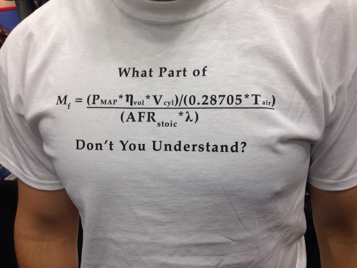
OE engine management systems are mass based, meaning that calculations are based on air mass. The air mass is either measured directly with a mass air meter, or calculated, based on a volumetric efficiency table and the basic speed density equation, proudly displayed here by Greg Banish of Calibrated Success.

(Not my favorite model, but certainly one of my favorite T-Shirts.)

Once the air mass is known, it can be divided by the target air fuel ratio to determine the fuel mass.

Once the fuel mass is known, the ECU needs a method of determining the injector pulse width that is required to deliver that fuel mass.

Enter the Injector Model

The injector model is a mathematical description of the dynamic response of the fuel injector.  In simple terms, it defines the pulse width that will deliver a given fuel mass.

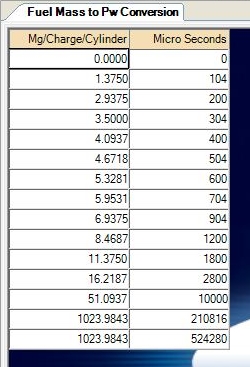
Chrysler’s method is based on the Fuel Mass to Pw Conversion table shown at the right.

In the left column, we have fuel mass per cylinder, per induction event. In the right column, we have the injector pulse width, in microseconds, that will deliver that fuel mass.

As you can see, it is a simple matter for the ECU to determine how long to pulse the injector.

Those of you who are paying attention will notice that the breakpoints are not spaced evenly, and while there is a great deal of resolution at low masses, the resolution is poor at higher masses.

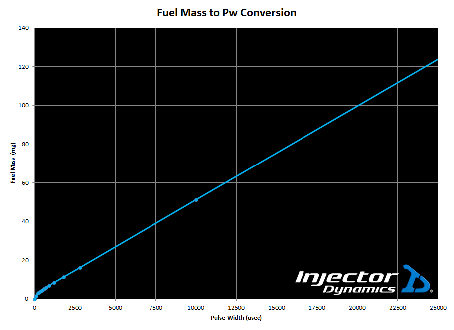
Those same astute readers have probably looked at a graph of the data, and been confused by what they saw. At least I hope they were, because I sure as hell couldn’t make any sense of this.

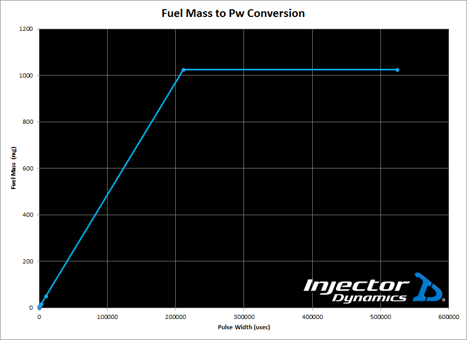
That is…unless I zoom in a bit to see what is happening. To do this, we only need to decide what to focus on. For starters, you may notice that the table goes all the way up to 524,280 microseconds. (524.28 milliseconds)

Those who have paid attention to your data logs in the past know that full throttle pulse widths normally fall between 15,000 and 20,000 microseconds. If you haven’t paid attention, that’s OK, you can still define a reasonable range with just a little bit of math.

For instance, knowing that RPM times 3.333 equals the time it takes (In microseconds) for a complete 720 degree engine cycle, we can quickly ascertain that at 6,000 RPM, a complete cycle lasts 20,000 microseconds. (6,000 X 3.333 = 20,000) and so a 20,000 microsecond pulse width at 6,000 RPM would equal a 100% duty cycle. This represents the largest possible pulse width at 6,000 rpm.

While the pulse width at the torque peak will certainly be higher, it’s a pretty safe assumption that our pulse width will never exceed 25,000 microseconds.

Focusing on the range from 0 to 25,000 microseconds, we get the following chart:

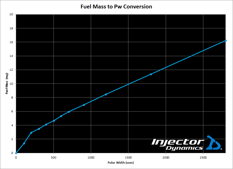
Now that we’re dialed in a little closer, a few things stand out. Most notable is that while we can draw a straight line from the 2,800 microsecond data point, all the way up to 25,000 microseconds, the data points below 2,800 microseconds deviate from a straight line, with the deviation increasing as pulse width decreases.

What we are looking at is two different ranges of the injector operation known as the linear operating range above 2,800 microseconds, and the lower non linear operating range below 2,800 microseconds. Since the non linear range is…well…non linear, it requires several data points to describe it accurately while the linear range could – at least in theory – be described with only two data points.

To further illustrate the lower non linear operating range, and its requirement for numerous closely spaced data points, I have zoomed in even further, displaying only the lower non linear operating range below 2,800 microseconds.

Now that we have a feel for what’s going on down low, if we turn our focus to the upper portion of the table, it makes a little more sense.

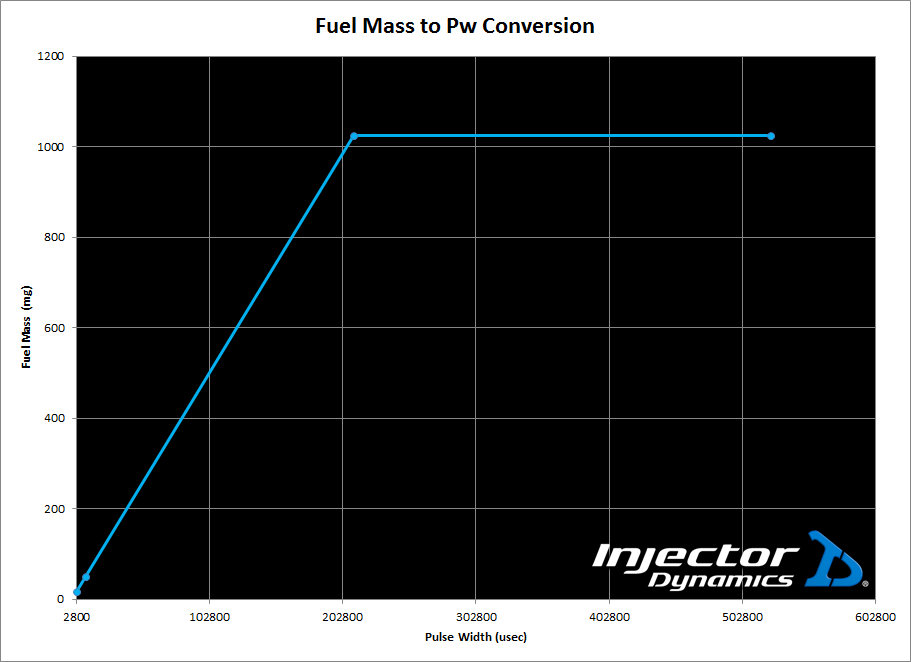
The graph below shows the data from 2,800 microseconds on up.

So I did say a “little” more sense, right?

Two things stand out. First is that we can draw a perfectly straight line through the data points at 2,800, 10,816, and 210,816 microseconds.

Second, the data point at 524,280, which shows the same fuel mass as the point below, is just filler.

The Joke’s on You

This raises an obvious question, which is “Why did they waste a third data point describing a straight line, and why did they waste the last data point when both of these could have been used to offer better resolution?” The answer is something to keep in mind as you foray into Chrysler tuning.

You will find lots of surprises in the Chrysler ECU that will leave you scratching your head, until you realize that some of it is just plain sloppy work.

I don’t say that for the sake of bashing Chrysler (I own one) I say that for the sake of making it clear to you, the tuner, that you will be forced to deal with some truly silly shit. I’m telling you this in advance so you don’t spend an evening trying to figure something out, only to find that the answer is akin to a bad knock knock joke.

Like this cute little table here.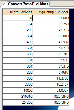

Look familiar? It should, because it is the exact same table that we started the article with, except that the variables have been swapped. Now instead of Converting Fuel Mass to Pw, we are converting Pw to Fuel Mass.

I told you there was some silly shit in here!

And certainly you are thinking “Why make us enter the same variables twice”

The answer…because if you don’t, the damn thing will not work properly, so make sure these tables are the exact inverse of each other, or you are going to have a bad day.

On With the Show

The tables above handle the basic conversion of fuel mass to pulse width, but these values are not constant, and so we need a few more variables to make sure we get the right answer as battery voltage and manifold pressure change.

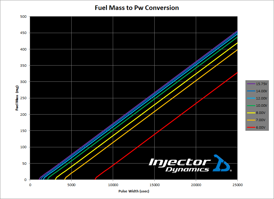
The chart below shows the raw flow vs pulse width of the stock Hemi injector at the 7 voltage points defined in the stock tune.

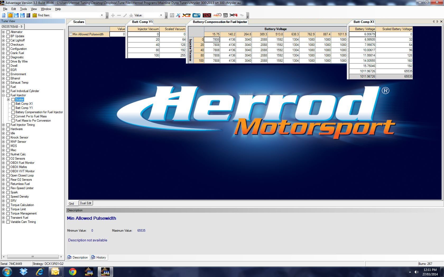
Looking at the battery compensation table to the right, you can see that we have a pulse width value in microseconds vs battery voltage on the X Axis, and vacuum in kPa on the Y Axis. In this case, the numbers remain constant across the Y Axis because the car is outfitted with a MAP referenced fuel pressure regulator which maintains a constant differential pressure across the injector.

Comparing the battery compensation table to the chart, we can see that the battery compensation value represents the “offset” of the flow vs pulsewidth curve, and the initiation of flow. For instance, at 6V, the compensation value is 7808, which is exacly the offset from the flow vs pulse width curve to zero.

Note that this is not always the case, as some cars use a return-less non MAP referenced fuel pressure regulator. This style of fuel system will maintain a constant pressure in the fuel rail, and so the differential fuel pressure across the fuel injector will change as the manifold pressure changes.